I'd rather have CABG surgery than go through this shit again.
read moreStudying for Final Exam
Separable equations: All you need to do is put the dx on one side and the dy on the other, grouped with their respective variables, and then you integrate both sides and you’re done.
Exact equations: Would be of the form M(x,y) + N(x,y)*dy/dx = 0. To make sure it’s exact, you would take M_y and N_x and check if they’re equal. Equality means it’s an exact equation. If that’s the case, take Psi_x = M and Psi_y = N. Integrate one of them, if you integrate Psi_x add f(y) and vice versa for Psi_y, then differentiate this integral with respect to the other variable (so differentiate integral(Psi_x)+f(y) with respect to y). Set this equal to the other equation (so Psi_y) and solve for what should now be f’(y). Then integrate to find f(y), and plug the result into the line where you introduced f(y), and you should be able to solve for y in that equation.
Integrating factors: If the equation is of the form dy/dx + a(t)*y=p(t), then the answer is pretty simple. We multiply both sides by eintegral(a(t)) and then we should see that the left hand side is the result of differentiating by the product rule, then we know we can integrate both sides and solve for y.
Homogeneous equation: If the order of all the terms is the same, we know it’s homogenous. It would be of the form M(x,y)dx+N(x,y)dy=0. Try to rewrite the equation to be of the form dy/dx = F(y/x). This may involve dividing everything by x or xn. Then substitute in u for y/x. We know dy=udx + xdx. Then we can plug in dy in terms of x and u into the dy in the equation. Then we should have everything in u’s and x’s, then we get all of each to either side, and then integrate and substitute back in y/x.
Bernoulli Equation: If you have a y that’s of a large order, say n, divide by yn and then solve as separable or homogenous.
————————————————————————————————————————
General Solution of Second Order Differential: Rewrite it as a characteristic equation, so y’’+5y’+6y = 0 becomes r2 +5r + 6 = 0. Solving for r gives possible values r1 and r2. Solution is y=c1*e(r1*t)+c2*e(r2*t).
Solving initial value: This will just have to be done by plugging in what they give you for y(0), and then you’ll have to differentiate the entire equation and then plug in y’(0) to get two equations that you can use to solve for c_1 and c_2.
Find answers with unreal roots: When solutions to the characteristic equation have an ‘i’, we need to use Euler’s formula e(it) = cos(t)+i*sin(t). So if we determine that the solution is e2it, then we would need to do c_1*(cos(2t)+i*sin(2t)).
Calculate imaginary roots: Use the quadratic formula to determine complex roots. 
Reduce imaginary solutions to real solutions: When you have two solutions, each of which involve i’s, you should take the sum and the difference of the two solutions and each of those should be real solutions. You can take out all the i’s and constant multipliers so that you have only your real.
Repeated Roots: This happens when b2-4ac=0. All we do here is take the one solution that the quadratic equation gives us, that is, e(-b/2a), and use that as one solution and use t*e(-b/2a) as another solution.
Method of Undetermined coefficients: First, solve the equation as if it were homogeneous. And then for each term on the right hand side, do undetermined coefficients.
1st: Write the characteristic equation.
2nd: Factor the equation into its two roots (if possible).
3rd: Say the coefficient of et on the right hand side is tn. Write out g to be A*tn+B*tn-1…etc.
4th: THEN LOOK AT THE COEFFICIENT OF THE EXPONENT OF et. If it’s a root, multiply g by how many times that root appears. So if the coefficient is 1, and (r-1)2 is a root, then multiply g by t2. DON’T ADD CONSTANTS.
5th: Write out g*f, the added multiplied t’s should already be in g.
6th: Create a table with the top row being STRICTLY BASED ON THE ORIGINAL RHS. So if you had t2*et, you would put that, then t*et, then et. You ignore all higher terms.
Variation of Parameters: First, we find the solutions of the equation as if it were homogeneous. We know that the solution should be of the form y=c_1*u1(t)y1+c_2*u2(t)y2. And we know that: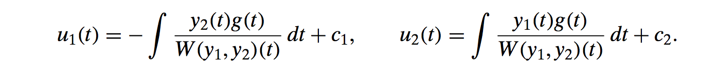
Where g(t) is the right hand side of the equation (the part that makes it non-homogeneous). And where W is the determinant of W = | y1(t) y2(t) |
| y’1(t) y’2(t) | .
Matrix inverse: Just augment with the identity, and then do row reduction to make the left hand matrix become the identity.
Linear Independence: Augment the matrix with all zeros, then do row reduction to see if an entire row can be made into all zeros (if it can, then they’re linearly dependent). If that doesn’t work, see if one row can be written completely as the other two. Essentially, linear dependence just means one row could be written as a linear combination of the other two. Row reducing should make it easy to spot if any are dependent.
————————————————————————————————————————
Solving for roots of 3rd or higher degree polynomial: Equations like this will be for nth order differential equations: r4 + r3 - 7r2 - r + 6 = 0. We need to practice long division of these beasts. Look at the common factors of the first and last coefficient, and attempt to long divide by (r-factor) for each factor until you get something that goes in evenly. Remember to try dividing out an r or r2 if you have r6-r2, for example. When you have a lonely r, or r2, you just treat it as if you have solution r=0. Remember if you have r2 that you have to do multiplicity 2, so you would have c*e0 + c*t*e0.
Writing solution for nth order differential equation: Once each of the roots have been found, all you need to do is write y=c_1*er1+c_2*er2+c_3*er3, etc. So just abstracting what we would do for the second order case.
Complex Roots for nth order: First, factor the equation as far as you can before tackling the complex roots. For example:
We can see that (r+1)(r-1) factors the left reduced form and (r+i)(r-i) factors the right one. We then use the real parts of Euler’s formula to figure out that the combined two solutions for the complex numbers are c_3*cos(t)+c_4*sin(t).
Undetermined Coefficients for nth order: First, we factor the equation, and generate the general solution. If there are roots with multiplicity greater than 1, then we multiply by t for each root after the first. So if you have (r-1)3, then you have et, tet, and t2et. Remember that we’re doing undetermined coefficients to find the particular solution to an equation, so we may need to add that to a general solution.
THE INFAMOUS 7.5
You’ll be given something like x’ = Matrix * x. You know that (Matrix - r*I)*(p1 \ p2) = 0.
- Subtract r from the diagonal of the matrix.
- Then take the determinant.
- Then find roots of this equation.
- Plug in the first root as r into the matrix with the -r’s on the diagonal,
- Multiply and solve for p1 in terms of p2.
- Write the column vector where the coefficient of p1 is on top and the other coefficient is on the bottom.
- Do the same for the other r.
- So if you your final solution is x=c1 (vector for r1)
er1*t+ c2 (vector for r2)er2*t.
————————————————————————————————————————
Things that really need some work:
Undetermined coefficients in general
Solving for roots of 3rd degree polynomial
Undetermined Coefficients for nth order
The last chapter. 7.5. NEEDS REVIEW. THERE WILL BE A PROBLEM ON THE TEST ON IT.
Anything else we’ve done since the last test that’s not mentioned above
————————————————————————————————————————
Refined study guide (based on things that need practice):
Exact equations
Practice undetermined coefficients right before test
The last chapter. 7.5. NEEDS REVIEW. THERE WILL BE A PROBLEM ON THE TEST ON IT.
————————————————————————————————————————
Little things to remember for each:
Integrating factor: You’ll have something of the form dy/dt +a(t)*y = p(t). You should multiply both sides by e^(integral(a(t)). Then you’ll see that the LHS is result of product rule; integrate both sides and solve for y.
Homogeneous: Rewrite of the form dy/dx=F(y/x), which may mean you have to divide by x or xn. Then substitute u=y/x, and dy=du*x+dx*u. Then get all u’s to one side and x’s to another, integrate, and sub back in.
Imaginary roots: Remember quadratic formula: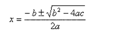
Repeated roots: Remember to multiply by t for every addition root you have.
Undetermined coefficients: Read the instructions above.
Matrix inverse: Augment with identity matrix, then row reduce until you get identity on original matrix.
Linear Independence: Augment with zeros, row reduce until you get close to identity. If you see that one row is a linear combination of the other two, then it’s dependent. Otherwise, independent.
Remember a lonely r solution (r*(r-1)*(r-2)) means that 0 is a solution, so corresponding e would be C*e0t.